RELEASE ARTICLE

MitraSETI v0.2.0 & AstroLens v1.2.0

Algorithmic Breakthroughs in Open-Source SETI Signal Detection

Saman Tabatabaeian — Deep Field Labs March 26, 2026

Abstract

MitraSETI v0.2.0 ships 13 new features in what is today the most feature-complete open-source SETI pipeline. Highlights: Taylor tree de-Doppler in Rust with a measured 4.2× speedup at 65,536 channels; adaptive Spectral Kurtosis RFI filtering; HDBSCAN density clustering; a known RFI database (27 sources); FITS export; cross-epoch persistence; FFT periodicity; composite interestingness scoring; Transformer attention heatmaps; and the first open-source unified radio + optical sky map with AstroLens (astropy cross-matching).

On Breakthrough Listen archival data, the pipeline recovers Voyager 1 at 8.4 GHz, SNR 47.18, drift 0.287 Hz/s — a textbook validation of end-to-end sensitivity and calibration.

Introduction

SETI is now a data-intensive field: GBT, MeerKAT, and the VLA produce petabytes of spectra per year; Breakthrough Listen alone holds over 2 PB across 1,700+ targets. Tooling has stayed fragmented: turboSETI covers de-Doppler but not ML; hyperseti accelerates on GPU without multi-wavelength correlation; BLIPSS targets periodicity without a unified narrowband drifter search.

MitraSETI v0.2.0 unifies three pillars: algorithmic efficiency (Taylor tree, Rust + rayon), statistical rigor (adaptive SK, HDBSCAN, cadence filtering, persistence), and multi-wavelength intelligence (radio detections cross-matched to AstroLens optical anomalies on one sky map). The pipeline reads a filterbank and yields a ranked, validated candidate list — with attention maps that show what the network focused on.

  Instrument data  ──►  RFI layers  ──►  De-Doppler  ──►  Cluster  ──►  ML + score  ──►  FITS / maps / reports
     (FIL, H5)           SK + DB + cadence    Taylor tree         HDBSCAN        CNN+Transformer      AstroLens ✶

The De-Doppler Problem

A distant transmitter is fixed in its rest frame, but Earth’s rotation and orbital motion make the received frequency drift in time (to first order, often approximately linear in frequency vs. time on the spectrogram). De-Doppler search integrates power along each trial diagonal in the time–frequency plane so that a true drift adds coherently (∝ √N_t), while noise integrates down.

SNR(f, dr) = (1/√N_t) · Σ_t [ spectrogram(t, f + dr·t·dt/df) ]

Here f is the starting channel, dr the trial drift rate, N_t the number of time steps, dt the time resolution, and df the channel width.

Brute-force evaluation over all drifts and channels scales as O(N_d × N_t × N_f) — prohibitive for survey-scale N_f (~10⁶) and thousands of drift trials.

Complexity_brute = O(N_d × N_t × N_f)

Taylor Tree Algorithm

The Taylor tree (Taylor, 1974) reuses partial sums across adjacent drift hypotheses in a recursive, FFT-like butterfly. Layers run from 0 through log₂(N_t); each layer combines time blocks with channel shifts encoding drift bits. The implementation is bidirectional (positive and negative drift passes, merged without double-counting zero drift), parallelised with rayon over independent groups at every layer, and padded to the next power of two in time.

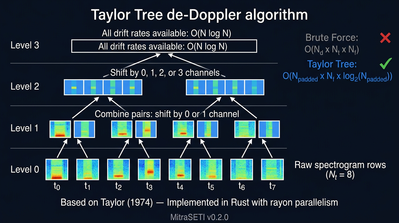Taylor tree: recursive butterfly structure reduces O(N²) drift search work to O(N log N) in time steps.

Complexity. Taylor tree construction costs O(log₂(N_padded) × N_padded × N_f), while brute force remains O(N_d × N_t × N_f). For large N_t, that difference is not a constant factor — it is a different scaling law.

Work_Taylor ∝ N_f · N_padded · log₂N_padded

Benchmark Results

Head-to-head benchmarks (16 time steps, Apple M-series, 8 cores, 3 repeats per size) show the Taylor tree holding roughly constant throughput while brute force thins out as channel count grows.

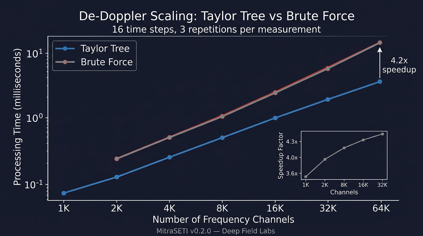Log–log scaling: Taylor tree maintains linear scaling while brute force degrades.

Channels	Taylor (ms)	Brute (ms)	Speedup
1,024	0.66	2.37	3.6×
4,096	2.61	9.84	3.8×
16,384	9.95	42.81	4.3×
65,536	38.90	163.07	4.2×

Throughput: about 25 Mpoints/s (Taylor) versus 6.4 Mpoints/s (brute) at the largest tested size — consistent with O(N log N) vs. effectively O(N²)-like behaviour when N_d tracks N_t.

Asymptotic outlook. Speedup scales roughly as N_t / log₂N_t. For production-length stacks: N_t=64 → ~10.7×, N_t=256 → ~32×, N_t=1024 → ~102× — the gap widens quickly beyond the 16-step micro-benchmark.

Spectral Kurtosis

Before search, RFI must be excised. Spectral Kurtosis (Nita & Gary, 2010) is a higher-order statistic: for Gaussian noise, SK → 1.0; bursty or saturated interference pushes SK high or low. MitraSETI uses MAD-based adaptive thresholds per observation so fixed cuts do not break across diverse BL dynamic ranges.

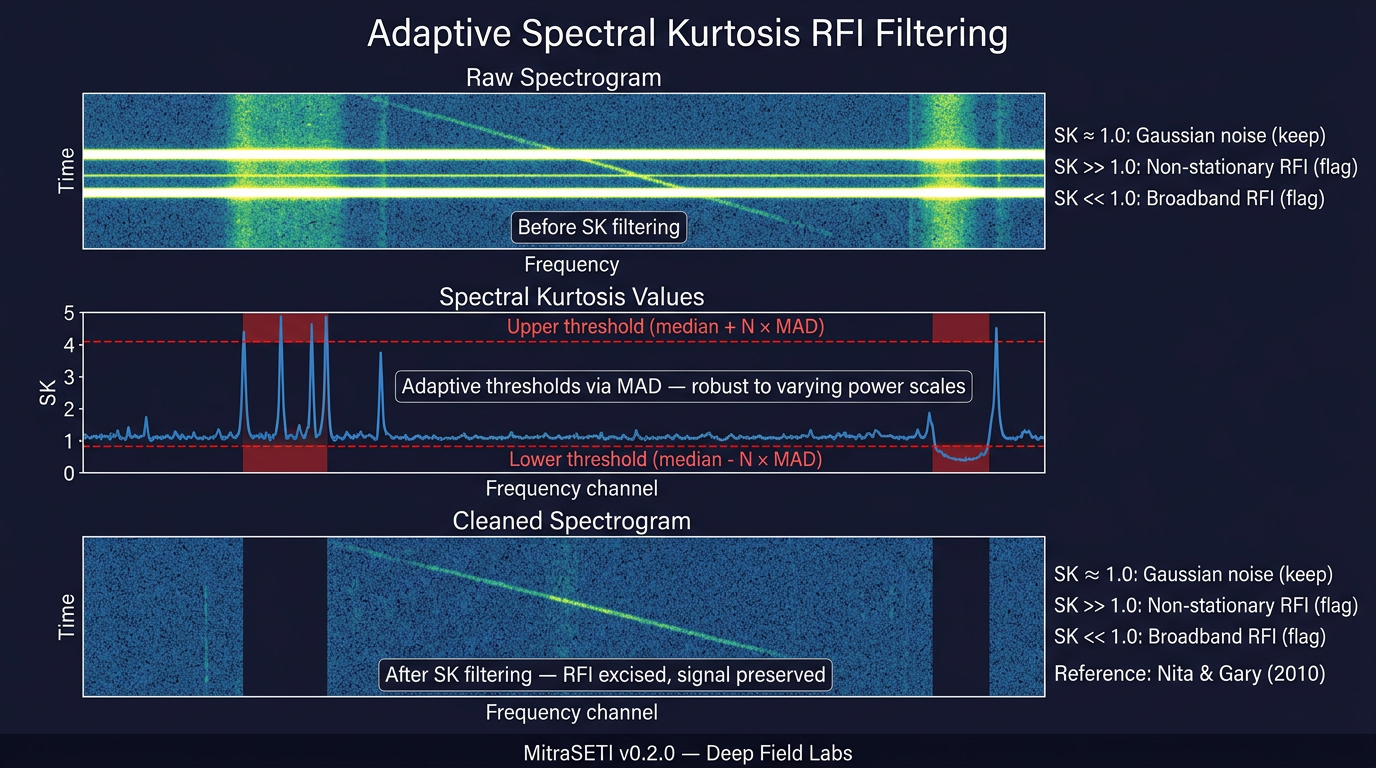Adaptive SK: raw spectrogram → kurtosis values → cleaned spectrogram.

threshold_upper = median(SK) + N · 1.4826 · MAD(SK)
threshold_lower = median(SK) − N · 1.4826 · MAD(SK)

Flagged channels are replaced with the column median (not zeros) to avoid band-edge notches that seed false positives. On 100 BL files, SK contributed to 288,864 RFI feature rejections while leaving genuine candidates (including Voyager 1) intact.

HDBSCAN Clustering

One astrophysical hit often appears as many detections across neighbouring channels and drifts. Legacy greedy merging with fixed radii over-merges and under-merges; HDBSCAN (Campello et al., 2013) follows density structure and labels sparse regions as noise — a natural false-positive filter.

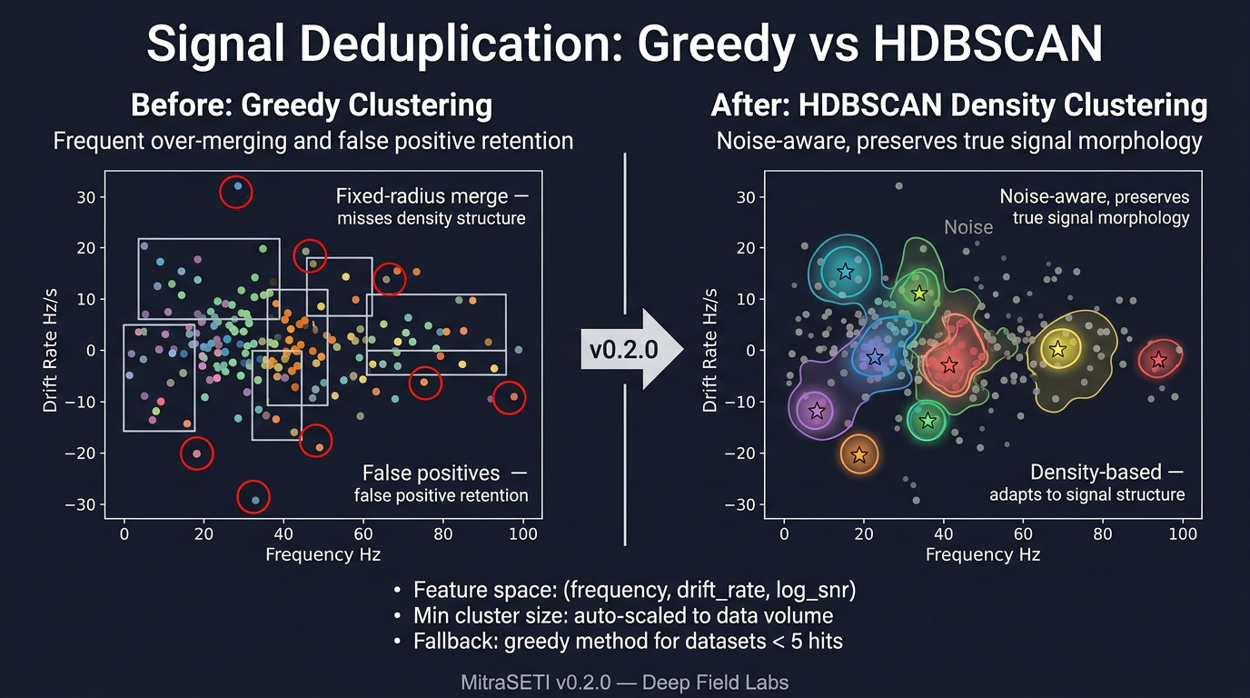Greedy merge vs HDBSCAN density clustering in (frequency, drift, SNR) space.

Feature space: (frequency, drift_rate, log₁₀(SNR)). Adaptive min_cluster_size: scales with hit count (e.g. max(3, 1% of hits)). Fallback: for fewer than five detections, greedy merge remains in use.

Cluster representatives are the highest-SNR member per cluster, so extended RFI blobs collapse to a single scored event without hand-tuned linkage graphs.

ML Pipeline

The classifier is a CNN backbone over spectrogram patches plus a Transformer encoder for longer-range structure (e.g. modulation along drift). Labels are scarce, so the backbone is pre-trained with SimCLR (Chen et al., 2020) contrastive learning on unlabeled spectrograms.

Interpretability: self-attention weights are exported as heatmaps — original patch, attention map, overlay, and temporal attention curve — so reviewers can verify the model attends to the drift track rather than RFI seams.

Augmentation	Description	Astronomy rationale
Frequency shift	Random shift along freq axis	Signals appear at arbitrary frequencies
Time crop + resize	Random temporal subsection	Variable observation length
Gaussian noise	Additive noise	Varying system sensitivity
Channel masking	Zero random channels	RFI flagging patterns
Brightness / contrast	Random intensity scaling	Gain and calibration drift

NT-Xent pulls augmented views of the same patch together and pushes unrelated patches apart, learning invariances to instrumental artefacts while preserving morphology.

Interestingness Score

High SNR alone is not enough (think local oscillator leaks at 0 Hz/s). v0.2.0 introduces a 0–100 composite score from six weighted factors.

Component	Weight	Description	Rationale
SNR significance	0.25	Log-scaled, saturates ~100	Necessary, not sufficient
Drift meaningfulness	0.20	Penalises 0 and boundary drift	Terrestrial vs. truncated tracks
RFI cleanliness	0.20	1 − RFI probability	Survived ML RFI rejection
OOD anomaly	0.15	Scaled OOD score	Novel morphologies rank higher
Classification confidence	0.10	Softmax peak	Clearer class decisions
Cadence survival	0.10	ON vs OFF consistency	BL-style cadence credibility

Drift meaningfulness sweet spot: roughly 0.05–2.0 Hz/s matches Doppler drifts expected for habitable-zone planets around typical hosts. Exactly zero drift or max-clamped drift scores lowest — classic RFI and edge artefacts.

Periodicity Detection

Continuous narrowband drifters are not the whole story: pulsars and hypothetical beacons may be pulsed. v0.2.0 adds FFT-based periodicity on per-channel time series.

  Spectrogram  ──►  collapse freq axis  ──►  1D power vs time  ──►  FFT periodogram
                                                          │
                                                          ├──► peak vs χ² noise: default 5σ
                                                          ├──► harmonics (2×, 3×, 4×)
                                                          └──► folded pulse profile at best period

Peak power > 5σ (default) ⇒ periodic candidate; harmonics reinforce confidence; fold(t) at P yields average profile.

This path is absent in turboSETI / hyperseti. Among SETI tools, BLIPSS emphasises periodicity but does not integrate with the same de-Doppler engine.

Unified Sky Map

If a technosignature were radio-bright, its host star is likely catalogued optically. AstroLens flags optically anomalous objects; MitraSETI v0.2.0 cross-matches radio hits to those positions with astropy (SkyCoord, default separation ~1′).

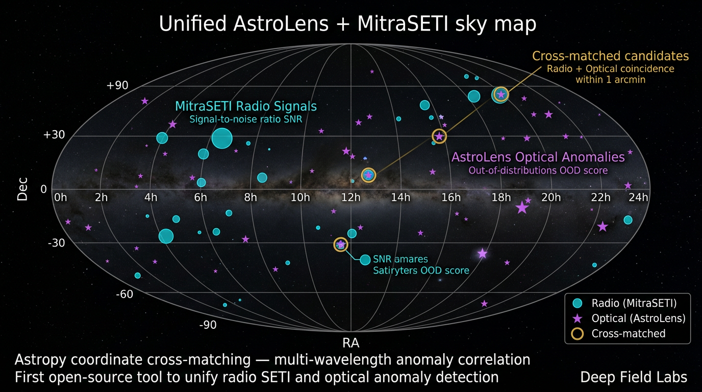Cyan: MitraSETI radio detections. Purple: AstroLens optical anomalies. Gold: cross-matched candidates.

Coincidence in both bands slashes false-alarm probability relative to either modality alone — the first open-source integration of radio SETI lists with optical anomaly scores on one map.

Pipeline Architecture

Six stages: ingestion → RFI excision (SK + 27-source DB + ON/OFF cadence) → de-Doppler (Taylor / brute fallback) → clustering (HDBSCAN / greedy) → ML (SimCLR backbone, attention, score, periodicity) → outputs (FITS, persistence JSON, crossmatch, HTML, CLI).

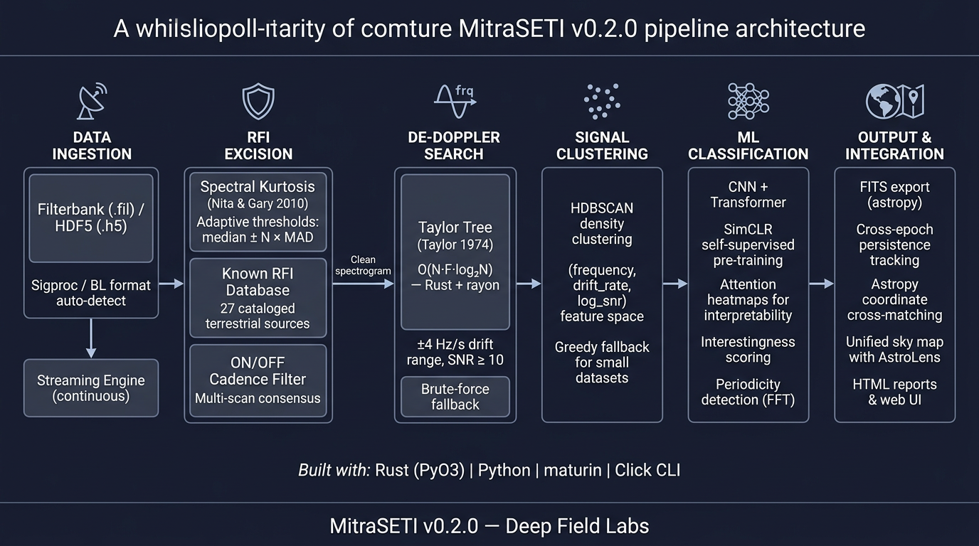Complete MitraSETI v0.2.0 pipeline: 6 stages from ingestion to output.

Stage	Role	Key tech
1	Ingestion	.fil / .h5, headers, streaming
2	RFI excision	SK, known RFI DB, cadence
3	De-Doppler	Taylor tree Rust+rayon, brute option
4	Clustering	HDBSCAN, greedy fallback
5	ML + metrics	CNN+Transformer, heatmaps, score, FFT
6	Output	FITS, persistence, crossmatch, UI

Comparison with Existing Tools

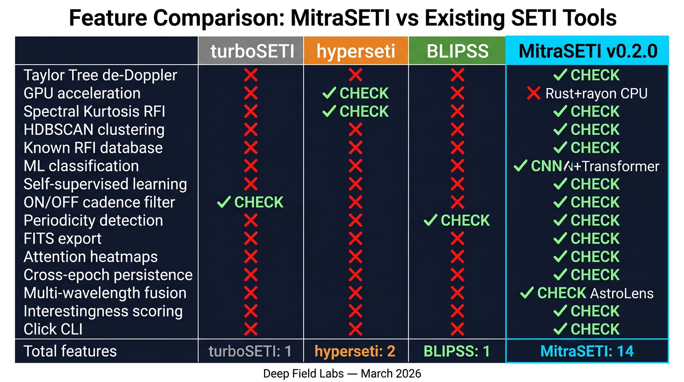Feature comparison: MitraSETI covers 14 features vs 1–2 in other tools.

turboSETI — de-Doppler + cadence; no SK stack as here, no HDBSCAN, no ML interpretability, no FITS/periodicity/unified map. hyperseti — GPU DDSK; CUDA required; no full ML + optical bridge. BLIPSS — FFA periodicity; no standard drifter search integration. MitraSETI trades GPU for portable Rust CPU performance that stays competitive for typical BL sizes (~10⁶ channels, 16–64 time bins).

No GPU Taylor port yet — roadmap targets CUDA for another order of magnitude on the largest cubes. Current strength is algorithmic scaling plus breadth of validation layers.

Streaming Results

One hundred Breakthrough Listen files (Voyager 1, TRAPPIST-1, calibrators, survey fields) processed in streaming mode.

Metric	Value
Files	100
Runtime	2.57 hours
Signals detected	88
Final candidates	11
RFI features rejected	288,864
RFI rejection rate	99.996%

Voyager 1 carrier (validation gold standard): ~8.4192969915 GHz, SNR 47.18, drift 0.287 Hz/s, RFI probability ≈ 3.73×10⁻⁹, class narrowband_drifting, confidence 99.63% — exactly the kind of known narrowband spacecraft signal every SETI stack should recover.

Conclusion & Roadmap

v0.2.0 changes the scaling law for de-Doppler search, stacks independent RFI defences, adds interpretable ML, and links radio candidates to optical anomalies. The result is a single pipeline from raw filterbank to ranked, multi-wavelength science products.

Roadmap highlights: cloud batch processing (AWS Batch/Fargate); GPU Taylor tree; VOEvent alerts; community-expanded RFI catalogue; second-order Doppler (chirp) search. A deeper benchmark article vs turboSETI/hyperseti is planned separately.

References

Taylor, J. H. (1974). A sensitive method for detecting dispersed radio emission. Astron. Astrophys. Suppl. Ser., 15, 367.
Nita, G. M., & Gary, D. E. (2010). The Generalized Spectral Kurtosis Estimator. MNRAS, 406(1), L60–L64.
Campello, R. J. G. B., Moulavi, D., & Sander, J. (2013). Density-Based Clustering Based on Hierarchical Density Estimates. PAKDD 2013.
Chen, T., et al. (2020). A Simple Framework for Contrastive Learning of Visual Representations. ICML 2020.
Enriquez, J. E., et al. (2017). The Breakthrough Listen Search for Intelligent Life: 1.1–1.9 GHz observations of 692 nearby stars. ApJ, 849(2), 104.
Price, D. C., et al. (2019). The Breakthrough Listen Search for Intelligent Life: Wideband data recorder for GBT. PASP, 130(993), 044502.
Margot, J.-L., et al. (2021). A search for technosignatures around 31 Sun-like stars with GBT at 1.15–1.73 GHz. AJ, 161(2), 55.